One of the limitations of Python, as compared to R, is the lack of statistical packages in Python. If you want to fit complicated models such as mixed models or survival models, R packages such as survival and lme4 are an easy way to solve such problems. However, no such packages exist in Python. R code generally doesn’t play nice when productionizing machine learning models. A powerful alternative is to use the Bayesian package pystan in Python, which basically fits any imaginable statistical model.

In this blog post I will demonstrate how to fit a complex mixed model using pystan. Suppose that we want to study the trend in average rainfall across 50 states over the last 10 years. The model I am going to fit is a generalized linear mixed model (GLMM) with uncorrelated random intercept and random slope. The model can be specified as:

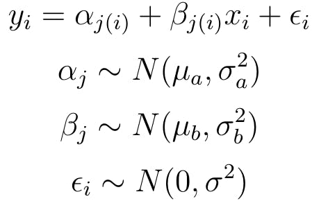Where \(y_i\) is average rainfall, \(x_i\) is calendar year, \(\alpha_j\) is random intercept and \(\beta_j\) is random slope.

First, let’s simulate some data.

states = ["AL", "AK", "AZ", "AR", "CA", "CO", "CT", "DC", "DE", "FL", "GA", 
          "HI", "ID", "IL", "IN", "IA", "KS", "KY", "LA", "ME", "MD", 
          "MA", "MI", "MN", "MS", "MO", "MT", "NE", "NV", "NH", "NJ", 
          "NM", "NY", "NC", "ND", "OH", "OK", "OR", "PA", "RI", "SC", 
          "SD", "TN", "TX", "UT", "VT", "VA", "WA", "WV", "WI", "WY"]

years = list(range(2010, 2020))

from random import seed, gauss
from collections import defaultdict

seed(1234)

intercept_mu, intercept_sigma, slope_mu, slope_sigma, error_mu, error_sigma = 20, 5, 0.05, 0.2, 0.1, 5

simulated_data = defaultdict(list)

for i, state in enumerate(states, 1):
    intercept = gauss(intercept_mu, intercept_sigma)
    slope = gauss(slope_mu, slope_sigma)
    for j, year in enumerate(years, 1):
        error = gauss(error_mu, error_sigma)
        simulated_data["state"].append(state)
        simulated_data["year"].append(year)
        simulated_data["intercept"].append(intercept)
        simulated_data["slope"].append(slope)
        simulated_data["error"].append(error)
        simulated_data['state_numeric'].append(i)
        simulated_data['year_numeric'].append(j)
        simulated_data["rainfall"].append(intercept + (slope * year) + error)


import pandas as pd

simulated_data_df = pd.DataFrame(simulated_data)

simulated_data_df.head(20)

Here is how the data looks like: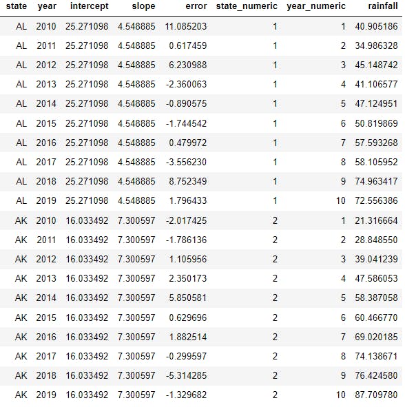

In real world you would only see the columns state, year and rainfall, I have added intercept, slope and error columns to illustrate the data generating process. The columns state_numeric and year_numeric are the required format by pystan. Here is how the \( rainfall = 40.90\) for the state of AL & year 2010 or year_numeric = 1 is generated:

\(rainfall =intercept +slope * year + error\)

\(40.90 = 25.27 + 4.548 * 1 + 11.085\)

Where \(25.27\) is drawn from \(N(20, 5)\), \(4.548\) is drawn from \(N(5, 2)\), and \(11.085\) is drawn from \(N(0.1, 5)\). The data generating process is fully specified and therefore it is straightforward to forecast rainfall over the next 10 years. Here is the estimate of the distribution of rainfall forecast for the state of AL for year 2025 or year_numeric = 16:

\(rainfall_{AL2025} \sim N(25.27 + 4.548 * 16, 5)\)

In part 2 of this blog post, I will demonstrate how to fit a mixed model using pystan and the data generated above. Stay tuned!

PS: The cover image is somewhere in central Oregon!